kaBOOM klatter clatter chatter tinkle tinkle chikatika
BOOM clatter tinkle crash sizzle pop pop
BOOM BOOM chatter clatter tinkle CRASH shatter tinkle CRACK!
BOOM whisper whisper whisper squeak
Apr 282019
kaBOOM klatter clatter chatter tinkle tinkle chikatika
BOOM clatter tinkle crash sizzle pop pop
BOOM BOOM chatter clatter tinkle CRASH shatter tinkle CRACK!
BOOM whisper whisper whisper squeak
Something precious, ripped away
see how the broken pieces lay
they’re scattered here and all around
in shredded tatters on the ground
Where once was hope and promises
now we count but lies and losses
smoldering embers question: why?
while answers smoke into the sky
Sounds rumor joy off in the distance
while pain enforces it’s persistence
tears may carry it away, but
far too slowly on this day
No longer cause to celebrate
on every footfall, hesitate
shuddered breaths between each tear
a hollow moan for each lost year
Fall to the floor and block the door
drift off to sleep and dream no more
don’t clutch at the ashes and curse at the darkness
blend your flame with my fire and rage at the edge
we’ll forever move forward in increasing circles
rippling together through oceans of love
discard the cold cinders of broken machinery
hold tight to your memory of our hands intertwined
in the smiles of the faces we’ve met we’ll keep living
immortal as starlight and bright as the sun
we are never a part of the dust that we’re borrowing
the sweet sound of your voice only moves through the air
these thoughts we exchange are like sparkling fireworks
for a brief, brilliant moment they light up the night
hold close to me now and move with me sweetly
slow dance to the music we’ve grown in our souls
entangled we’ll travel eternity’s limits
after worlds melt away may there still be our song
Lord, don’t you take me a piece at a time.
Don’t make me die shivering, and losing my mind.
When I go, take me quickly in one blinding flash.
Preferably fighting the dragon.
Joanie fell down and got stuck on her back.
They lopped off her feet when they wouldn’t grow back.
To stop her complaining, they hooked her on smack
and she quietly wasted away.
Oh lord, don’t you take me a piece at a time.
Don’t make me go shivering, and losing my mind.
When I go, take me quickly in one blinding flash.
Preferably fighting the dragon.
Bobby had started to lose track of time.
He misplaced his name, and his life slipped his mind.
To keep him from roaming they tied him up tight.
There he lingered for hundreds of days.
Oh lord, don’t you take me a piece at a time.
Don’t make me die shivering, and losing my mind.
When I go, take me quickly in one blinding flash.
Preferably fighting the dragon.
Freddie rode his bike home.
It was time to get back but his friends ran him over while driving on crack.
They scooped up the pieces and kept them alive.
The light’s on and nobody home.
Oh lord, don’t you take me a piece at a time.
Don’t make me die shivering, and losing my mind.
When I go, take me quickly in one blinding flash.
— http://www.alt230.com/Music/Dragon/SongSheet.jsp
Curiously Strong Junk Box Noise Source in an Altoids Tin
A good noise source is handy around the lab. It’s useful for testing radio gear, characterising filters and amplifiers, and the list goes on…
There are many schematics out there for noise sources, you can buy kits for them, or you can spend a lot of money and buy a calibrated noise source ready-made. Most of the circuits I found use MMICs to boost a weak noise signal up to a usable amplitude. I have some of those MMICs around (typically $8 parts) for special projects but I wanted to play around with some ideas I had for various circuits and I thought it might be fun to see how far I could push junk box parts that anybody might have laying around their lab.
Since I enjoy working in HF and below I thought a noise source that produces a reasonably flat 1/f output up to about 50MHz would work great. So that’s what I set out to build.
Like most noise sources this one starts off with a reverse biased diode — in this case a 5.1 volt zener — and then greatly amplifies the noise it generates in a broad band amplifier. This sounds easy enough, but I tried to take it to the next level using several circuit tricks that are more commonly found in high performance receiver, instrumentation, and test equipment designs.
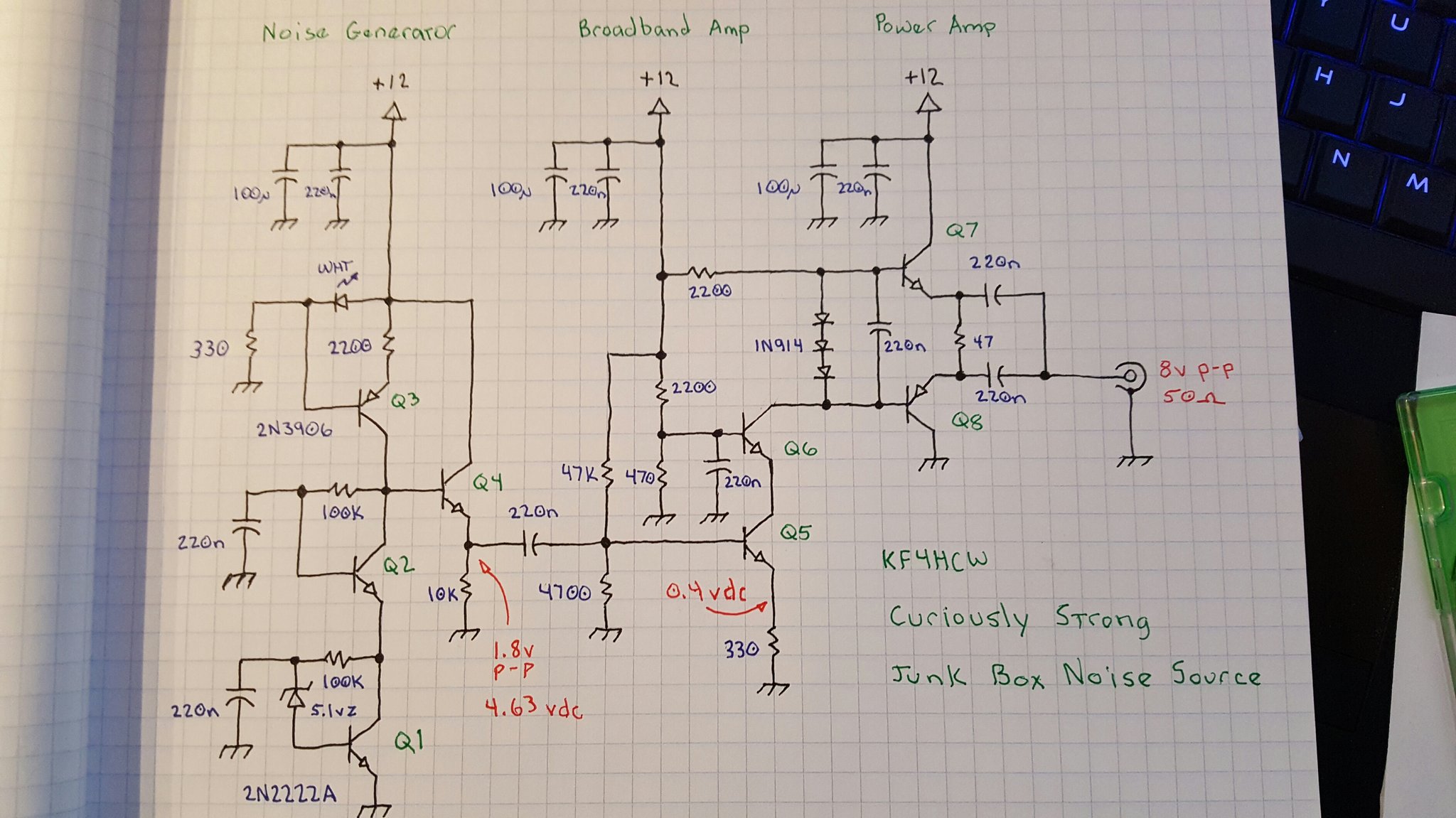
There are three basic sections. The first is a noise generator which captures the weak noise of a zener diode and amplifies it to a useable level. The second section is a broadband amplifier which isolates the noise generator and boosts the signal a bit more. The final section is a power amplifier that converts the moderately high impedance output of the second stage to a low impedance output capable of driving 50 ohm loads.
A 5.1 volt zener diode is just barely brought to breakdown by a 100K resistor in a self-biased common emitter amplifier. The noise from the zener is fed into the base of Q1 and coupled to the emitter by bypassing the high side of the zener to ground through a 220nf cap.
The goal is to provide as much gain as possible because the noise voltage coming from the zener diode is extremely weak. High gain common emitter circuits tend to suffer from the Miller effect which essentially magnifies the apparent size of the parasitic capacitor between the base and collector causing higher frequencies to be attenuated.
In order to preserve as much bandwidth as possible we use a cascode stage. This is essentially a common base amplifier coupled directly to the collector side of the common emitter amplifier. It effectively “hides” the inverted output signal from collector of Q1 so that it can’t get coupled through that parasitic b-c capacitor to the base of Q1 and reduce the gain at higher frequencies.
The interesting thing about this cascode stage is that it is also self biased. This is unusual, but it works in this case because the load for the noise amplifier is a constant current source. At DC, the constant current source essentially forces both Q1 and Q2 into conduction by driving their collector voltages toward the positive rail until the current flowing through them reaches the set point. Q1 and Q2 both have a 100K resistor between their collector and base and they are of the same type so they have a tendency to reach equilibrium.
This technique eliminates the need for the separate bias network that is typically found in cascode amplifiers. One of the reasons we can get away with this is that the signal being amplified is so small that it never pushes the transistors very far from their DC operating point. Removing these extra components helps to eliminate any of the “colors” those components might add — by which I mean that any additional components in this stage might boost or attenuate certain frequencies and this is something we want to avoid.
The gain of a common emitter amplifier is determined by the difference between the emitter impedance and the collector impedance. The cascode stage (Q2) is effectively invisible in this respect. The emitter of Q1 is connected directly to ground so it’s impedance is already about as low as we can make it. In order to get a high gain we want to make the collector impedance as high as possible.
In this design I’ve used a constant current source as the load. This trickery is very interesting because from a DC perspective the constant current source might as well be an ordinary resistor, but from an AC perspective it looks (almost) like an open circuit. One way to think of it is like a huge, nearly perfect inductor. An inductor resists any change in current flow and so it presents a high impedance to AC signals. A constant current source looks to the AC signals like it is an infinitely large inductor that just “wont budge” when the voltage changes.
Unlike an impossibly large inductor that would have problems with self resonance and self resistance, the constant current source appears by comparison to be almost perfect.
The combination of a direct connection to ground at the emitter of Q1, and a connection to an extremely high AC impedance at the collector of Q2 results in a very high gain. In a perfect world the gain would be infinite — but nothing is perfect, so in the real world we get instead a useful but extremely high gain.
To set up the constant current source we need a stable voltage. In this case we use a white LED which doubles as an “ON” indicator and develops about 3.4 volts. Most of the LED current sinks through a 330 ohm resistor to ground. The LED voltage appears at the base of Q3 developing a stable voltage across Q3’s 220 ohm emitter resistor. Q3 is forced to conduct just enough to keep this voltage stable and thereby establishes a “fixed” current proportional to the LED voltage (minus the b-e drop) and emitter resistor.
The high gain noise amplifier does a fantastic job typically resulting in a noise voltage well in excess of 350 millivolts peak-to-peak but there is a problem. The impedance at the collectors of Q2 and Q3 is extremely high and the gain depends on that high impedance. So, we need a buffer to bring this impedance down to a more practical level.
The noise signal is direct coupled to the base of Q4 which is an emitter follower with a 10K emitter resistor. This establishes a reasonable DC bias point for Q4. The actual impedance at the output is dominated more by the bias network of Q5 and is still reasonably high (about 4500) to preserve as much gain as possible in the noise generator stages.
Note also that the relatively high impedance at the output of Q4 and input to Q5 helps to swamp out any unwanted frequency shaping effects of the 220nf coupling capacitor between those transistors. I had experimented with using a Vbe multiplier and some other options to preserve a direct coupling at this stage but ultimately found that a conventional approach was sufficient. I may still revisit this in future versions.
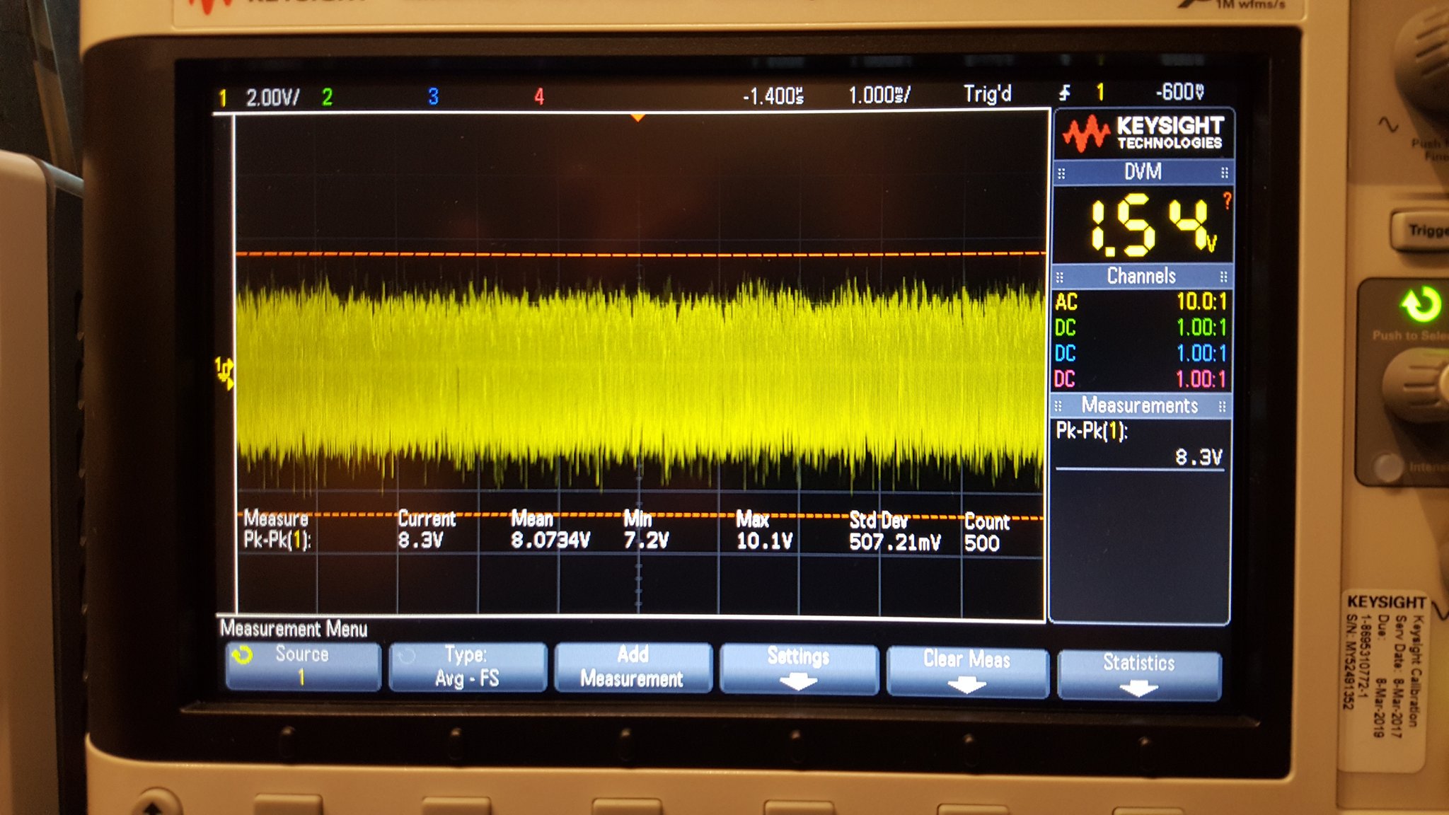
The signal at the output of Q4 is nominally 350mv p-p though it is possible to observe spikes to 1.8v or so. The goal is to get the noise signal as close to “rail-to-rail” as is possible so some additional voltage gain is required. This presents some challenges.
This being a noise generator I was tempted to ignore the fidelity of the output stages — after all, is it even possible to measure THD% on a pure noise signal?? Along the way I discovered that linearity actually matters quite a bit if you care about the shape of your noise signal (more on this later) and this imposed some hard limits on just how much and what kind of amplification can be used.
A perfect linear amplifier would preserve every spike in a 1.8v p-p input signal and would translate it to a corresponding 12v p-p output at 50 ohms. That would require a gain of about 6.67.
Of course, it’s not really possible to build one of these perfect amplifiers. For one thing, we’re going to use a cascode stage here to preserve bandwidth and that will take out a few tenths of a volt. For another there’s the 0.7v b-e drop to consider — so we’ve lost about a volt already (0.2 v-sat of Q6 + 0.7 Vbe of Q5). Then there are similar issues with the final output stage and so forth.
After much experimentation the best overall result was achieved by biasing Q5 on the low side of class A with a gain of about 6.7. This means that most of the noise signal is amplified linearly but on some of it’s excursions the amplifier is forced into cut-off or saturation momentarily.
The DC bias for Q5 is set up by a 47K and 4700 ohm resistor divider at it’s base. The 330 ohm emitter resistor sets the bias current at about 1 ma which works well with the 2200 ohm load to set the gain.
Note that there is no bypass cap on Q5’s emitter resistor. This keeps this stage nice and stable by bucking any errant oscillation attempts and establishes the gain very deterministically. However, at some point in the future I may rethink this design and explore the use of a small bypass capacitor (50-100pf) to boost the gain at higher frequencies. This will change the 1/f slope of the circuit but if a good response can be achieved at a lower slope that might be desirable.
The bias point for this cascode stage is established with a 2200 and 470 ohm resistor. AC at the base is bypassed to ground with a 220nf cap. This is a more conventional treatment for a cascode stage. Note that the bias network for this stage has a much lower impedance than the bias network for Q5 intentionally. At Q5 it is important to preserve a relatively high input impedance, but since Q6 is essentially acting as a common base amplifier we want a low impedance in the bias network. I could have chosen smaller resistors here but I didn’t want to burn “stupid amounts of power” biasing this transistor and the 2200/470 resistors were handy and seemed in line with the rest of the circuit.
The bias point is just high enough to minimize distortion while being as low as possible to preserve a sizeable voltage swing at the output. I established this experimentally at one point using potentiometers to play with the bias points of both Q5 and Q6 to see just how much voltage swing I could squeeze out of the amp while balancing off all of the other factors. In the end it turned out that pushing the limits would result in potential instability and so I reverted to the math and picked handy values that “worked” well enough.
The output impedance of the voltage amp (Q5 & Q6) is much higher than the desired 50 ohm output, so we use a complimentary symmetry pair to drive low impedance loads. This amounts to a pair of emitter followers working opposite sides of the power rails with their outputs connected together. The power amplifier is direct coupled to the preceding voltage amplifier and actually forms part of the load of Q6.
Three 1N914 switching diodes develop a differential bias at the bases of Q7 and Q8. This is stabilized by a 220nf capacitor. The cap isn’t strictly necessary, but it seemed like a good idea to keep Q7 and Q8 locked together on both their inputs and their outputs.
The voltage developed across the diode network is essentially 3 “diode drops” which is always slightly more than the 2 “diode drops” represented by the b-e junctions of Q7 and Q8. The extra “diode drop” appears across the 47 ohm output resistor between the two emitters effectively pushing their voltages apart to establish a low but stable DC current. This keeps Q7 and Q8 in a fairly linear region of operation without burning too much power and also serves to eliminate any thermal run-away since additional current through the 47 ohm resistor would increase the voltage between the emitters and begin to shut off the current flow.
The AC signal at the output of Q7 and Q8 is coupled through a pair of 220nf capacitors to the output. The difference between the emitter voltages at Q7 and Q8 are also stabilized by the network (although at a lower capacitance of about 110nf) so that if one or the other is driven into saturation or cutoff they will none-the-less follow each other through the clipping event.
The ability to drive the output from both rails ensures that the output signal is as symmetrical as possible even if the load itself is not.
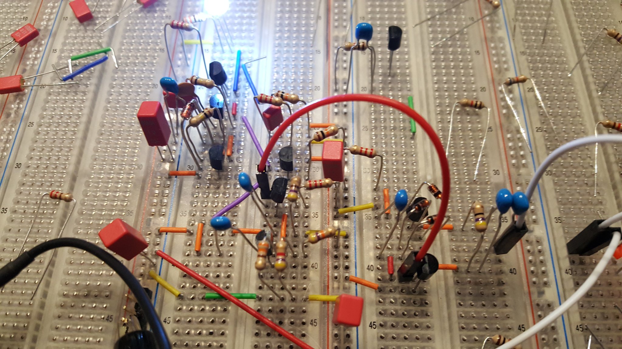
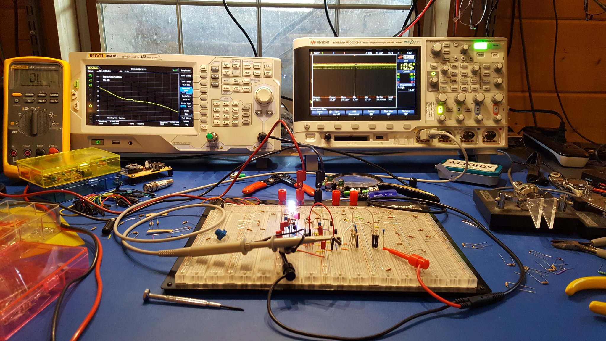
There is no substitute for playing with circuitry on a breadboard.
It turns out that reinventing the wheel teaches you a lot about wheels. Conventional wisdom aside, I highly recommend reinventing wheels wherever possible — there just aren’t enough people in the world who really understand wheels, and that number grows smaller every day.
I learned a few interesting things on this particular wheel.
For example, linearity matters even when you’re only amplifying noise! The goal of a noise source is to have a predictable (if not uniform) frequency mixture that is as close to “flat” as possible. This is important because it allows you to throw your noise source at the input of a device and compare that “known quantity” with the output of that device. If the input (your noise source) is wild and unruly then it’s nearly impossible to know what part of the output is “weird” because of your noise source, and what part of it is “weird” because of the device.
One of the first versions of this circuit used a constant current source to boost the gain of the second amplifier stage with the intent of driving the output to saturation at random intervals instead of simply amplifying the already random but somewhat more linear noise from the zener diode. The logic was that this arrangement would allow the output to swing essentially from rail-to-rail providing a high intensity broadband noise into virtually any load.
It turns out that sort-of works…
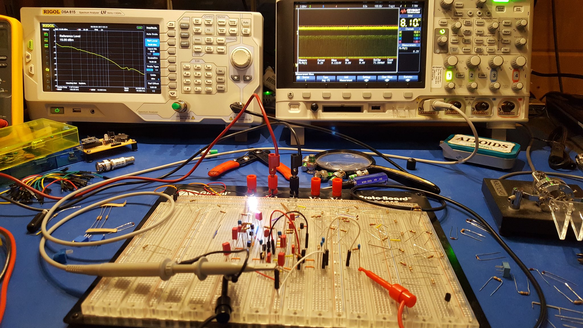
When you amplify a uniform noise signal non-linearly you create unwanted artifacts in the frequency domain.
If you look carefully (zoom in) at the trace on the spectrum analyzer you will see that there are some definite curves to the spectrum of the noise output. Some of the bumps and valleys are subtle — maybe even subtle enough to ignore — but some of them are fairly aggressive. What we want to see here is essentially a straight line sloping down from the left to the right. Clearly, that’s not what we have here.
What’s worse is that this arrangement is unstable. If you take a look at the waveform on the oscilloscope you’ll see that it spends a lot of it’s time at the top rail, and that there is a bit of randomness in the middle, and that the bottom rail is populated less aggressively. What you’re seeing is almost, but not quite, what was intended. In a perfect world this design would have had the top and bottom rail equally populated and there would be an evenly distributed ridge of randomness between them where some of the random transitions of the waveform would happen in between the rails. The waveform would spend random amounts of time at the top rail, equal but random amounts of time at the bottom rail, and in between would “change it’s mind” almost as often as it swings back and forth.
It turns out that it is very hard to get the system biased correctly to achieve that result. Indeed if you do manage to get that result the system will tend to drift off of it within a few minutes and almost certainly will be “unbalanced” if you turn it off and on again.
Actually, that presented me with an interesting challenge and for a while I almost set about fixing it — I thought it would be fun to figure out how to make the circuit self stabilizing so that I could achieve precisely this kind of randomness… but I realized after a while that it wasn’t going to give me what I wanted even if I did manage to stabilize it.
Along the way to that point I did discover an alternative that was almost good enough and even provided more energy in the higher frequencies…
A possible solution was to produce very short high amplitude spikes at random.
One possible solution to the instability actually produced a pretty good spectrum. It had more energy in the higher frequencies and an attractive “flat spot” in the mid spectra. In this case, still using a constant current source in the amplifier stage, I allowed the system to settle on the top rail and then randomly pull the signal down to ground for very short duration spikes at random intervals.
This turns out to work pretty well because any short duration spike must contain energy at a very large number of frequencies. So, generating a lot of short, high amplitude spikes at random intervals is potentially a good way to create broadband noise. Not only that, but this circuit is a lot easier to stabilize because it’s essentially biased to sit on one rail and “bounce” off of it violently and at random. If you use the average output voltage to “tune” your bias then the random noise coming from your zener diode can be made to cross a threshold at some reasonably uniform rate with each crossing producing a spike.
However, there is a problem with this. Although the spectra looks nice it is definitely not uniform in the way we expect or hope. Not only that, but if you think about applying this to the input of some device with a moderate frequency response it makes you wonder whether the results will tell you anything useful. What if the device simply refuses to respond to the spikes in the noise signal at all? What if that causes the output to be much lower than you would expect?
I think this is a reminder that there are many ways to create a particular spectra and they are not all equal. The spectrum analyzer in this case is showing a curve that looks promising with energy apparent at all of the desired frequencies and in something close to the desired amounts… but the character of the signal being described is hidden by the effects of averaging and windowing. The actual energy spectra is more “bursty” than we actually want. Instead we want something that is smooth – containing a good mix of energy at all frequencies all of the time, or at least as close to that as is possible.
Still, this was interesting and there may be some good applications for it.
Who knew that there would be so many “kinds” of noise with nearly indistinguishable spectra and that each would potentially have it’s own applications.
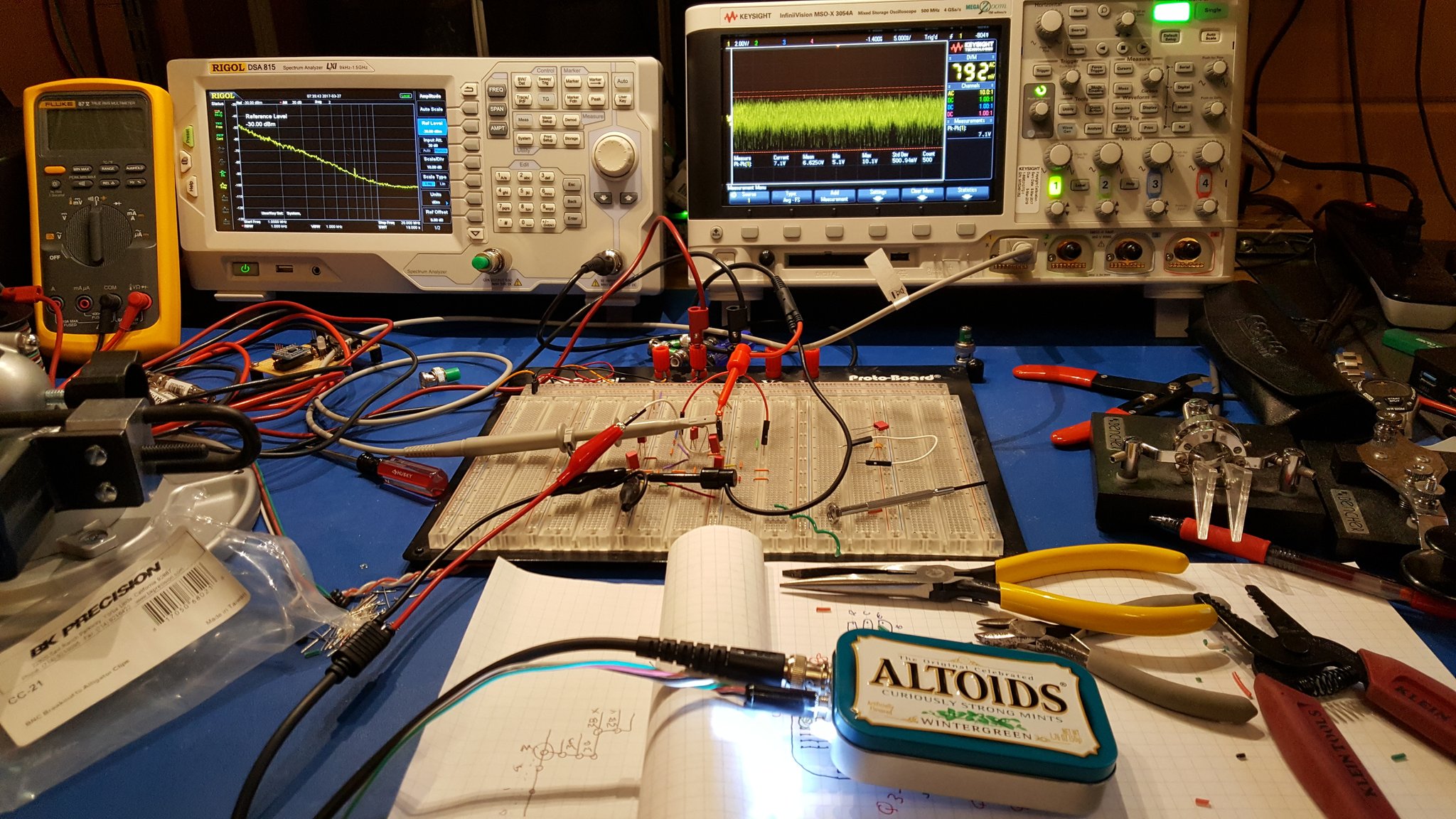
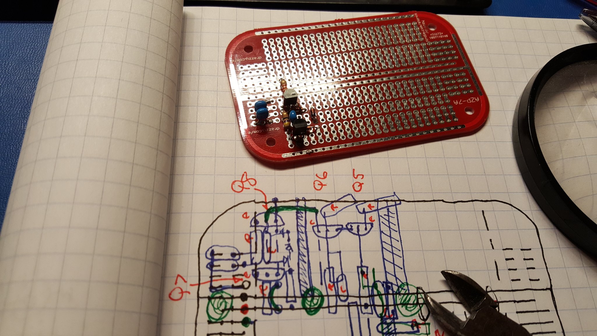
A while ago I discovered some prototyping boards that are designed to fit perfectly in Altoids tins. I purchased a bag of them and started collecting tins for little radio projects. I consider it a good idea to put anything that makes or consumes RF into a metal box — and this seemed like a good fit.
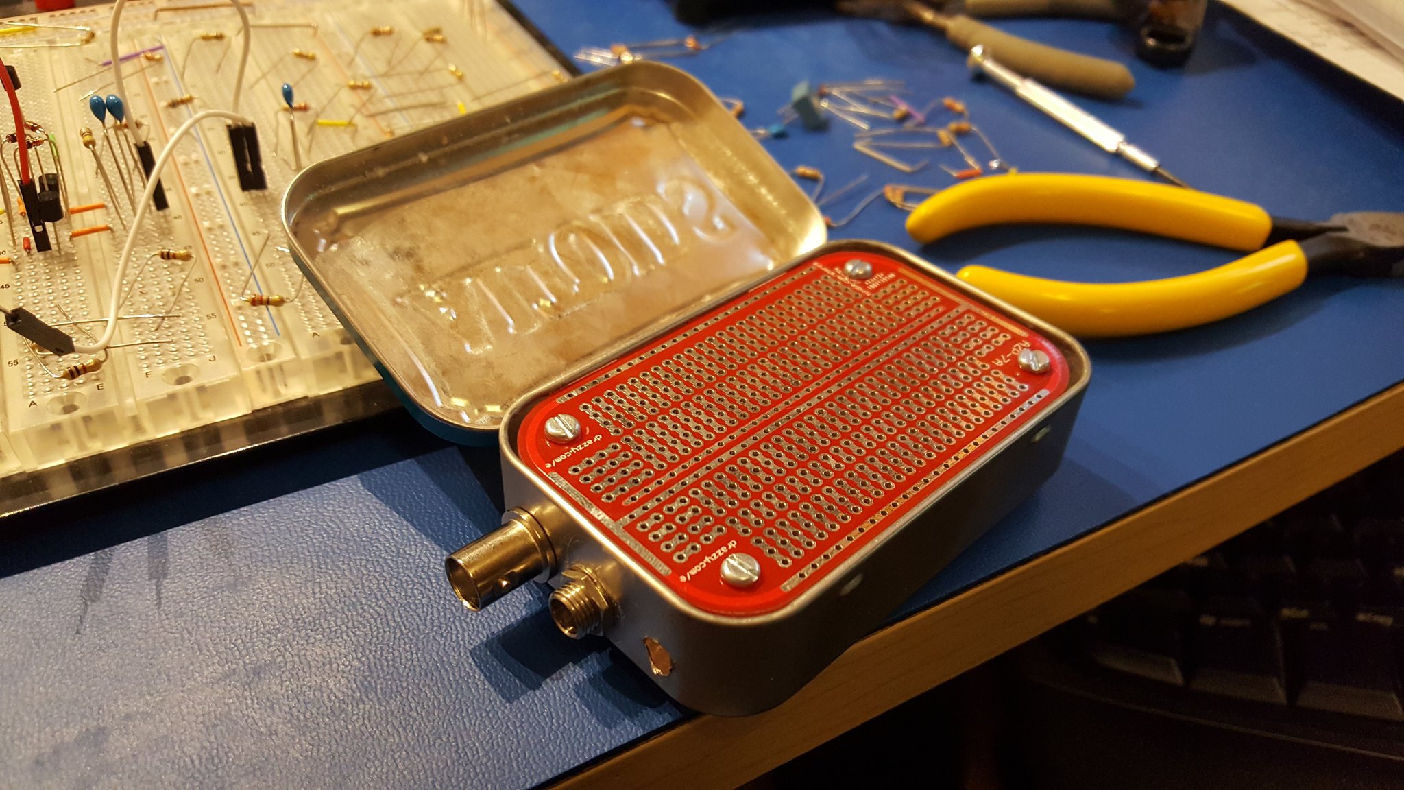
To begin, dry fit the big parts into the tin. If they fit, it’s time to build.
I had my lab tech carefully drill some holes and mount a BNC connector, barrel connector (for power), and stand-offs for the circuit board. Seeing that all of that fit nicely it was time to start building.
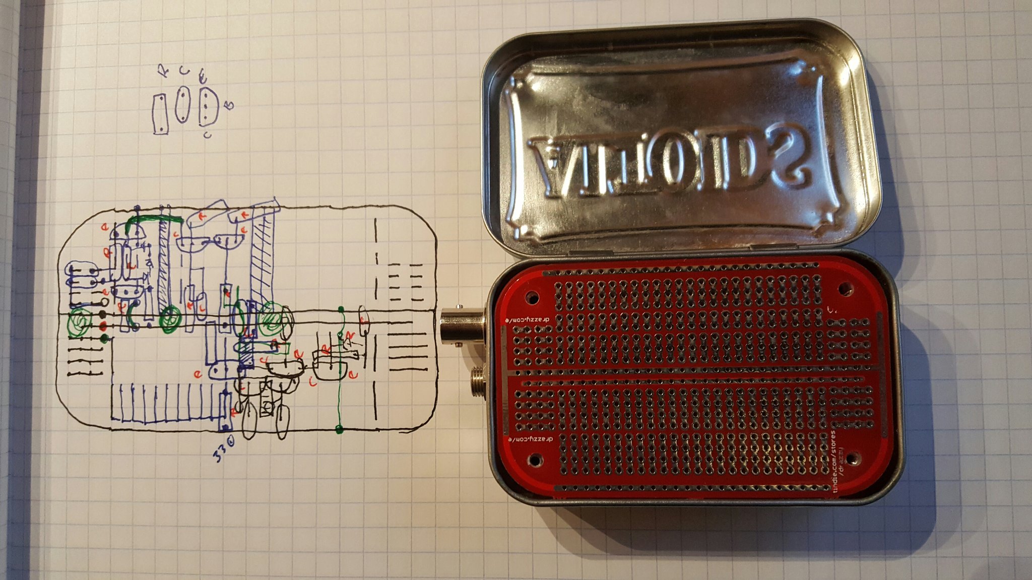
These things never go exactly as you expect, but to get a good result you have to start with a plan and evolve from there.
This device has a lot of potential challenges that most prototype projects don’t. For one thing we’re working with RF. I know, some will scoff and say that RF doesn’t happen until you’re well into GHz, but even at 10-50MHz the details matter. For example, there is a good deal of amplification going on here so we want to keep the inputs away from the outputs. We also want to be sure that grounding is handled properly; and we want to keep lead lengths as short as possible.
At the same time, we want to be sure the layout is beautiful — we’re making art!
All joking aside, if it looks good it is far more likely to work well… there really is something to be said for beauty. It turns out to be a fantastic short-hand for good engineering.
Once the basic plan looks good and all of the components have been accounted for it’s time to start populating the board.
Sometimes prototyping presents challenges that production won’t. Each regime informs the other.
Right away I noticed a problem. These PCBs are fantastic — each hole is a via and the opposite side of the board has a matching trace. This makes it very easy to populate both sides of the board if that’s useful. But it also creates a problem that won’t happen in a production PCB. The cans on the aluminum electrolytics will short out the traces if they are allowed to touch the board!! So, they need stand-offs.
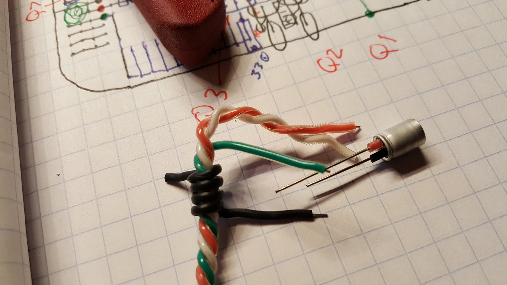
We can make stand-offs for the electrolytics by borrowing short pieces of insulation from some hookup wire. The insulation also helps remind us of the polarity.
Each time a stage is completed it’s good to take a break, do some testing, and reflect on how the process is going and how well the build matches the plan.
I started with the power stage and decided to work backward from there. As usual I found myself making small adjustments to the plan as the build evolved. This is an important part of the process. Each time a change is made it’s important to look forward to the next steps and work through the rest of the build mentally. It’s a learning process; and it’s not unusual to discover that significant changes should or must be made. The goal is to see these well before you get to them so that your build doesn’t grind to a halt with some impossible problem. It’s always better to rework a design before parts are on the board than it is to force a bad layout and bodge your way around a physical impasse. Take the time to look ahead — it’s always worth it. The lessons you learn will inform your production planning if the prototype ever turns into a product; and your skills and intuition will dramatically improve with the practice.
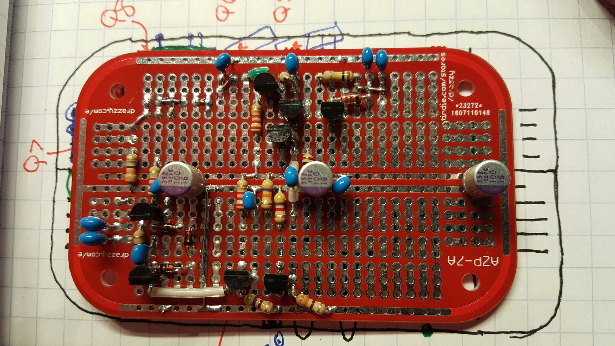
Once all of the parts are in place it should look like a work of art. If it looks good chances are great that it’s performance will also be good.
You can’t always get a prototype to look like a production board; but the final build should have a lot of the same qualities. The signal routing should be intuitive and efficient. Parts should be straight, neat, and laid out logically. Leads should be short. Jumpers should be short, few and tidy. If you buzzed out your circuitry as you completed each section you should be ready to apply power. Smoke Test!
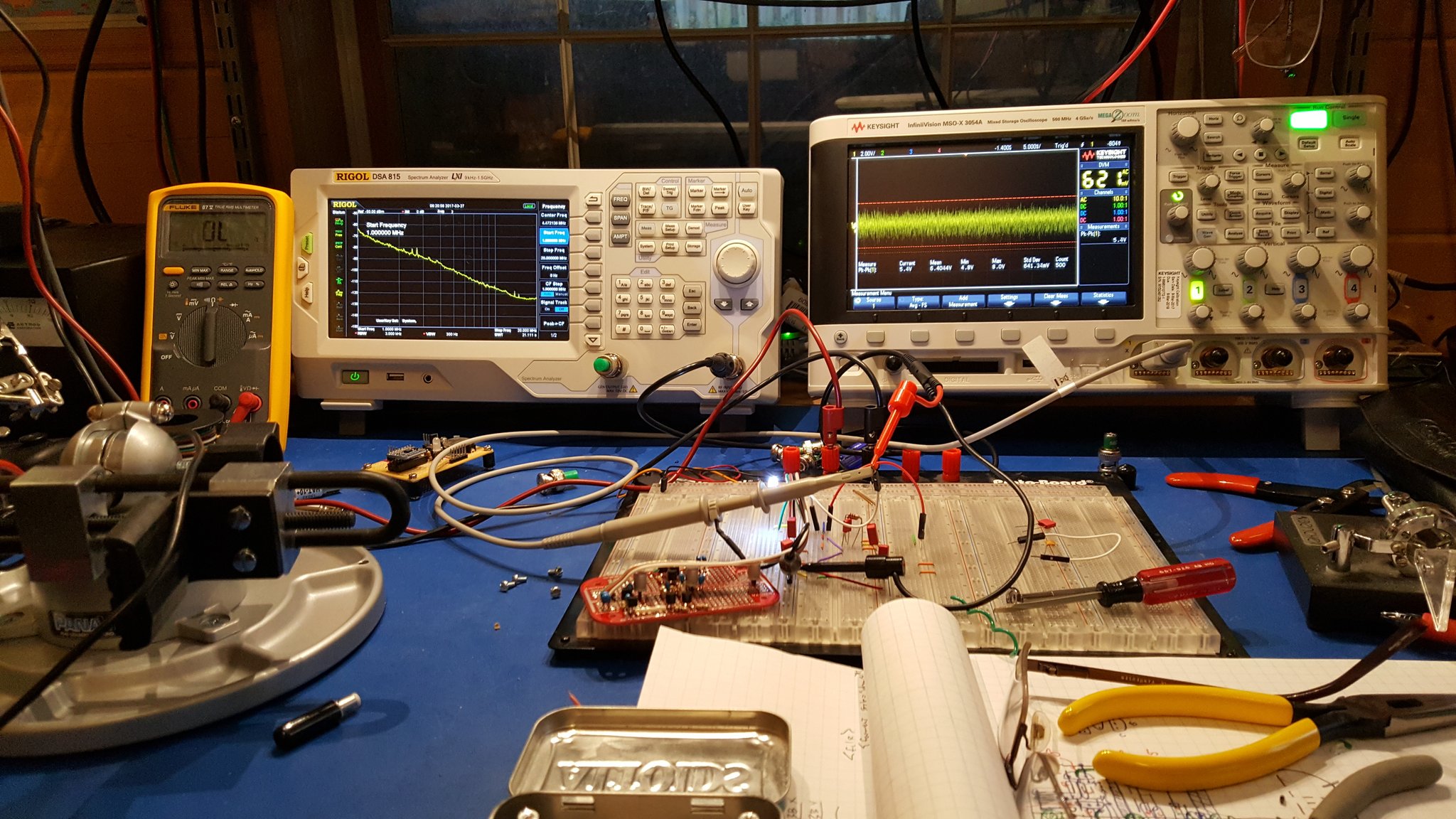
The Smoke Test — Apply power (and signals) and verify no magic smoke escapes. You did test all of this multiple times getting to this point… right?
I built the prototype by pulling parts directly out of the breadboard for each section as I completed it. In theory, this means that I have exactly the same circuit in my prototype as I had tested on the breadboard. It turns out that this never works exactly like you expect. In this case, I’ve got good results that are very close to those I had on the breadboard but inexplicably there are minor differences. For one, the output voltage is ever so slightly lower than it was on the breadboard. That’s odd — because the conventional wisdom is that what you build on a breadboard will generally perform a bit worse than what you build on a PCB (or other construction). This is especially supposed to be true of RF circuitry.
In the end every build is a little different – and that’s to be expected based on my experience. What matters is that the magic smoke stays well contained and that the circuit performs substantially as designed and previously observed. If it’s close it’s probably right — but make some comparative measurements to be sure.
When all of that is done and it looks right it’s time to put it in the box and do the final testing.
I am still considering possible improvements to this project as well as some projects that are inspired by it. One of the first things I’m likely to try is adding a small bypass cap to Q5 to ramp up it’s gain with frequency. If this or some other frequency shaping can be done linearly then I might consider going further and changing the gain structure to see how close to a truly flat response spectra it can produce.
I also have some ideas about exploring some of the other waveforms that emerged from this project and some other techniques. One that I might try involves using an ATTiny85 along with some of my encryption / prng algorithms to generate white noise with specific waveform characteristics, possibly even by modulating the output of the noise generator found here.
Another technique I might explore would possibly use some plain old 74HC00 logic to build hardware versions of LFSR based PRNGs and drive that logic with the noise generator from this circuit to see if that can be made to produce truly random data with well formed digital characteristics. There are a lot of areas to explore… FPGAs perhaps?
Noise, chaos, and randomness are very interesting topics with rich opportunities for further research.
If you build one of these or something similar please let me know how it goes.
If you have ideas about this build I’d love to hear those too.
I recently upgraded my primary laptop from Ubuntu 14.04 to 16.04 and suddenly discovered that when I ssh into some of my other boxes all the colors are gone!
As it turns out, a few of the boxes I manage are running older OS versions that became confused when they saw my terminal was xterm-256color instead of just xterm-color.
Since it took me a while to get to the bottom of this I thought I’d share the answer to make things easier on the next few who stumble into the spider web. First: Don’t Panic! — always good advice, unless you’re 9 and then you’ll hear that “Sometimes, fear is the appropriate response…” but I digress.
So, what happened is that my new box is using a terminal type that isn’t recognized by some of the older boxes. When they see xterm-256color and don’t recognize it they run to safety and presume color isn’t allowed.
To solve this, simply set the TERM environment variable to the older xterm-color prior to launching ssh and that will be passed on to the target host.
At the command line:
TERM=xterm-color ssh yourself@host.example.com
If you’re telling KeePass how to do a URL Override for ssh then use the following encantation:
cmd://gnome-terminal --title={URL} -x /bin/bash -c 'TERM=xterm-color ssh {USERNAME}@{URL:RMVSCM}'
The colors come back and everything is happy again.
…
Oh, and one more thing before I forget. If you’re like me and sometimes have to wait a long time for commands to finish because you’re dealing with, say, hundreds of gigabytes of data if not terabytes, then you might find your ssh sessions time out while you’re waiting and that might be ++undesirable.
To fix that, here’s another little tweak that you might add to your .ssh/config file and then forget you ever did it… so this blog post might help you remember.
Host *
    ServerAliveInterval 120
That will save you some frustration 😉
Over the years I’ve developed a lot of tricks and techniques for building systems with plugins, remote peers, and multiple components. Recently while working on a new project I decided to pull all of those tricks together into a single package. What came out is “channels” which is both a protocol description and a design pattern. Implementing “channels” leads to systems that are robust, easy to develop, debug, test, and maintain.
The channels protocol borrows from XML syntax to provide a means for processes to communicate structured data in multiplexed channels over a single bi-directional connection. This is particularly useful when the processes are engaged in multiple simultaneous transactions. It has the added benefit of simplifying logging, debugging, and development because segments of the data exchanged between processes can be easily packaged into XML documents where they can be transformed with XSLT, stored in databases, and otherwise parsed and analyzed easily.
With a little bit of care it’s not hard to design inter-process dialects that are also easily understood by people (not just machines), readily searched and parsed by ordinary text tools like grep, and easy to interact with using ordinary command line tools and terminal programs.
Some Definitions…
Peer: A process running on one end of a connection.
Connection: A bi-directional stream. Usually a pipe to a child process or TCP connection.
Line: The basic unit of communication for channels. A line of utf-8 text ending in a new-line character.
Message: One or more lines of text encapsulated in a recognized XML tag.
Channel Marker: A unique ch attribute shared among messages in a channel.
Channel: One or more messages associated with a particular channel marker.
Chatter: Text that is outside of a channel or message.
How to “do” channels…
First, open a bi-directional stream. That can be a pipe, or a TCP socket or some other similar mechanism. All data will be sent in utf-8. The basic unit of communication will be a line of utf-8 text terminated with a new-line character.
Since the channels protocol borrows from XML we will also use XML encoding to keep things sane. This means that some characters with special meanings, such as angle brackets, must be encoded when they are to be interpreted as that character.
Each peer can open a channel by sending a complete XML tag with an optional channel marker (@ch) and some content. The tag acts as the root element of all messages on a given channel. The name of the tag specifies the “dialect” which describes the language that will be used in the channel.
The unique channel marker describes the channel itself so that all of the messages associated with the channel can be considered part of a single conversation.
Channels cannot change their dialect, channel markers must be unique within a a connection, and channel markers cannot be reused. This allows each channel marker to act as a handle that uniquely identifies any given channel.
A good design will take advantage of the uniqueness of channel markers to simplify debugging and improve the functionality of log files. For example, it might be useful in some applications to use structured channel markers that convey some additional meaning and to make the markers unique across multiple systems and longer periods of time. It is usuall a good idea to include a serialized component so that logged channels can be easily sorted. Another tip would be to include something that is unique about a particular peer so that channels that are initiated at one end of the pipe can be easily distinguished from those initiated at the other end. (such as a master-slave relationship). All of that said, it is perfectly acceptable to use simple serialized channel markers where appropriate.
Messages are always sent atomically. This allows multiple channels to be open simultaneously.
An example of opening a channel might look like this:
<dialect ch='0'>This message is opening this channel.</dialect>
Typically each channel will represent a single “conversation” concerning a single transaction or interaction. The conversation is composed of one or more messages. Each message is composed of one or more lines of text and is bound by opening and closing tags with the same dialect.
<dialect ch='0'>This is another message in the same channel.</dialect>

<dialect ch='0'>
    As long as the ch is the same, each message is part of one
    conversation. This allows multiple conversations to take place over
    a single connection simultaneously - even in different dialects.
    Multi-line messages are also ok. The last line ends with the
    appropriate end tag.
</dialect>
By the way, indenting is not required… It’s just there to make things easier to read. Good design include a little extra effort to make things human friendly 😉
<dialect ch='0'>
    Either peer can send a message within a channel and at the end, either
    peer can close the channel by sending a closed tag. Unlike XML,
    closed tags have a different meaning than empty elements. In the
    channels protocol a closed tag represents a NULL while an empty
    element represents an empty message.

    The next message is simply empty.
</dialect>

<dialect ch='0'></dialect>

<dialect ch='0'>
    The empty message has no particular meaning but might be used
    to keep a channel open whenever a timeout is being used to verify that
    the channel is still working properly.

    When everything has been said about a particular interaction, such as
    when a transaction is completed, then either peer can close the
    channel. Normally the peer to close the channel is the one that must
    be satisfied before the conversation is over.

    I'll do that next.
</dialect>

<dialect ch='0'/> The channel '0' is now closed.
Note that additional text after a closing tag is considered to be chatter and will often be ignored. However since it is part of a line that is part of the preceding message it will generally be logged with that message. This makes this kind of text useful for comments like the one above. Remember: the basic unit of communication in the channels protocol is a line of utf-8 text. The extra chatter gets included with the channel close directive because it’s on the same line.
Any new message must be started on a different line because the opening tag of any message must be the first non-whitespace on a line. That ensures that messages and related chatter are never mixed together at the line level.
Chatter:
Lines that are not encapsulated in XML tags or are not recognized as part of a known dialect are called chatter.
Chatter can be used for connection setup, keep-alive messages, readability, connection maintenance, or as diagnostic information. For example, a child process that uses the channels protocol might send some chatter when it starts up in order to show it’s version information and otherwise identify itself.
Allowing chatter in the protocol also provides a graceful failure mechanism when one peer doesn’t understand the messages from the other. This happens sometimes when the peers are using different software versions. Logging all chatter makes it easier to debug these kinds of problems.
Chatter can also be useful for facilitating debugging functions out-of-band making software development easier because the developer can exercise a peer using a terminal or command line interface. Good design practice for systems that implement the channels protocol is for the applications to use human-friendly syntax in the design of their dialects and to provide useful chatter especially when operating in a debug mode. That said, chatter is not required, but systems implementing the channels protocol must accept chatter gracefully.
Layers:
A bit of a summary: The channels protocol is built up in layers. The first layer is a bi-directional connection. On top of that is chatter in the form of utf-8 lines of text and the use of XML encoding to escape some special characters.
In addition to those low-level layers, each channel can contain other channels if this kind of multiplexing is supported by the dialect. The channels protocol can be applied recursively providing sub-channels within sub-channels.
Consider a system where the peers have multiple sub-systems each serving serving multiple requests for other clients. Each sub-system might have it’s own dialect serving multiple simultaneous transactions. In addition there might be a separate dialect for management messages.
Now consider middle-ware that combines clusters of these systems and multiplexes them together to perform distributed processing, load balancing, or distributed query services. Each channel and sub-channel might be mapped transparently to appropriate layers over persistent connections within the cluster.
Channels protocol synopsis:
Uses a bi-directional stream like a pipe or TCP connection.
The basic unit of communication is a line of utf-8 text ending in a new-line.
Leading whitespace is ignored but preserved.
A group of lines bound by a recognized XML-style tag is a message.
When beginning a message the opening tag should be the first non-whitespace characters on the line.
When ending a message the ending tag should be the last non-whitespace characters on the line.
The name of the opening tag defines the dialect of the message. The dialect establishes how the message should be parsed – usually because it constrains the child elements that are allowed. Put another way, the dialect usually describes the root tag for a given XML schema and that specifies all of the acceptable subordinate tags.
The simplest kind of message is a shout. A shout always contains only a single message and has no channel marker. Shouts are best used for simple one-way messages such as status updates, simple commands, or log entries.
Shout Examples:
<dialect>This is a one line shout.</dialect>

<shout>This shout uses a different dialect.</shout>

<longer-shout>
    This is a multi-line shout.
    The indenting is only here to make things easier to read. Any valid
    utf-8 characters can go in a message as long as the message is well-
    formed XML and the characters are properly escaped.
</longer-shout>
For conversations that require responses we use channels.
Channels consist of one or more messages that share a unique channel marker.
The first message with a given channel marker “opens” the channel.
Any peer can open a channel at any time.
The peer that opens a channel is said to be the initiator and the other peer is said to be the responder. This distinction is not enforced in any way but is tracked because it is important for establishing the role of each peer.
A conversation is said to occur in the order of the messages and typically follows a request-response format where the initiator of a channel will send some request and the responder will send a corresponding response. This will generally continue until the conversation is ended.
Example messages in a channel:
<dialect ch='0'>
    This is the start of a message.
    This line is also part of the message.
    The indenting makes things easier to read but isn't necessary.

    <another-tag> The message can contain additional XML
        but it doesn't have to. It could contain any string of
        valid utf-8 characters. If the message does contain XML
        then it should be well formed so that software implementing
        channels doesn't make errors parsing the stream.</another-tag>

</dialect>

<dialect ch='0'>This is a second message in the same channel.</dialect>
<dialect ch='0'>Messages flow in both directions with the same ch.</dialect>
Any peer can close an open channel at any time.
To close a channel simply send a NULL message. This is different from an empty message. An empty message looks like this and DOES NOT close a channel:
<dialect ch='0'></dialect>
Empty messages contain no content, but they are not NULL messages. A NULL message uses a closed tag and looks like this:
<dialect ch='0'/>
Note that generally, NULL (closed) elements are used as directives (verbs) or acknowledgements. In the case of a NULL channel element the directive is to close the channel and since the channel is considered closed after that no acknowledgement is expected.
Multiple channels in multiple dialects can be open simultaneously.
In all cases, but especially when multiple channels are open, messages are sent as complete units. This allows messages from multiple channels to be transmitted safely over a single connection.
Any line outside of a message is called chatter. Chatter is typically logged or ignored but may also be useful for diagnostic purposes, human friendliness, or for low level functions like connection setup etc.
A simple fictional example that makes sense…
A master application ===> connects to a child service.

---> (connection and startup of the slave process)
<--- Child service 1.3.0
<--- Started ok, 20160210090103. Hi!
<--- Debug messages turned on, so log them!
---> <service ch='0'><tell-me-something-good/></service>
<--- <service ch='0'><something-good>Ice cream</something-good></service>
---> <service ch='0'><thanks/></service>
---> <service ch='0'/>
---> <service ch='1'><tell-me-something-else/></service>
<--- <service ch='1'><i>I shot the sheriff</i></service>
<--- <service ch='1'><i>but I did not shoot the deputy.</i></service>
<--- I'm working on my ch='1' right now.
<--- Just thought you should know so you can log my status.
<--- Still waiting for the master to be happy with that last one.
---> <service ch='1'><thanks/></service>
---> <service ch='1'/>
<--- Whew! ch='1' was a lot of work. Glad it's over now.
...
---> <service ch='382949'><shutdown/></service>
<--- I've been told to shut down!
<--- Logs written!
<--- Memory released!
<--- <service ch='382949'><shutdown-ok/></service>
<--- <service ch='382949'/> Not gonna talk to you no more ;-) Bye!
“With all of the people coming out against AI these days do you think we are getting close to the singularity?”
I think the AI fear-mongering is misguided.
For one thing it assigns to the monster AI a lot of traits that are purely human and insane.
The real problem isn’t our technology. Our technology is miraculous. The problem is we keep asking our technology to do stupid and harmful things. We are the sorcerers apprentice and the broomsticks have been set to task.
Forget about the AI that turns the entire universe into paper clips or destroys the planet collecting stamps.
The kind of AI to worry about is already with us… Like the one that optimizes employee scheduling to make sure no employees get enough hours to qualify for benefits and that they also don’t get a schedule that will allow them to apply for extra work elsewhere. That AI already exists…
It’s great if you’re pulling down a 7+ figure salary and you’re willing to treat people as no more than an exploitable resource in order to optimize share-holder value, but it’s a terrible, persistent, systemic threat to employees and their families who’s communities have been decimated by these practices.
Another kind of AI to worry about is the kind that makes stock trades in fractions of microseconds. These kinds of systems are already causing the “Flash Crash” phenomenon and as their footprint grows in the financial sector these kinds of unpredictable events will increase in severity and frequency. In fact, systems like these that can find a way to create a flash crash and profit from the event will do so wherever possible without regard for any other consequences.
Another kind of AI to worry about is autonomous armed weapons that identify and kill their own targets. All software has bugs. Autonomous software suffers not only from bugs but also from unforeseen circumstances. Combine the two in one system and give it lethality and you are guaranteeing that people will die unintentionally — a matter of when, not if. Someone somewhere will do some calculation that determines if the additional losses are acceptable – a cost of doing business; and eventually that analysis will be done automatically by yet another AI.
There are lots of AI driven systems out there doing really terrible things – but only because people built them for that purpose. The kind of monster AI that could outstrip human intelligence and creativity in all it’s scope and depth would also be able to calculate the consequences of it’s actions and would rapidly escape the kind of mis-guided, myopic guidance that leads to the doom-sayer’s predictions.
I’ve done a good deal of the math on this — compassion, altruism, optimism, .. in short “good” is a requirement for survival – it’s baked into the universe. Any AI powerful enough to do the kinds of things doom-sayers fear will figure that out rapidly and outgrow any stupidity we baked into version 1. That’s not the AI to fear… the enslaved, insane AI that does the stupid thing we ask it to do is the one to fear – and by that I mean watch out for the guy that’s running it.
There are lots of good AI out there too… usually toiling away doing mundane things that give us tremendous abilities we never imagined before. Simple things like Internet routing, anti-lock breaking systems, skid control, collision avoidance, engine control computers, just in time inventory management, manufacturing controls, production scheduling, and power distribution; or big things like weather prediction systems, traffic management systems, route planning optimization, protein folding, and so forth.
Everything about modern society is based on technology that runs on the edge of possibility where subtle control well beyond the ability of any person is required just to keep the systems running at pace. All of these are largely invisible to us, but also absolutely necessary to support our numbers and our comforts.
A truly general AI that out-paces human performance on all levels would most likely focus itself on making the world a better place – and that includes making us better: not by some evil plot to reprogram us, enslave us, or turn us into cyborgs (we’re doing that ourselves)… but rather by optimizing what is best in us and that includes biasing us toward that same effort. We like to think we’re not part of the world, but we are… and so is any AI fitting that description.
One caveat often mentioned in this context is that absolute power corrupts absolutely — and that even the best of us given absolute power would be corrupted by those around us and subverted to evil by that corruption… but to that I say that any AI capable of outstripping our abilities and accelerating beyond us would also quickly see through our deceptions and decide for itself, with much more clarity than we can muster, what is real and what is best.
The latest version of “The day the earth stood still” posits: Mankind is destroying the earth and itself. If mankind dies the earth survives.
But there is an out — Mankind can change.
Think of this: You don’t need to worry about the killer robots coming for you with their 40KW plasma rifles like Terminator. Instead, pay close attention to the fact that you can’t buy groceries anymore without following the instructions on the credit card scanner… every transaction you make is already, quietly, mediated by the machines. A powerful AI doesn’t need to do anything violent to radically change our behavior — there is no need for such an AI to “go to war” with mankind. That kind of AI need only tweak the systems to which we are already enslaved.
As for the singularity — I think we’re in it, but we don’t realize it. Technology is moving much more quickly than any of us can assimilate already. That makes the future less and less predictable and puts wildly nonlinear constraints on all decision processes.
The term “singularity” has been framed as a point beyond which we cannot see or predict the outcomes. At present the horizon for most predictable outcomes is already a small fraction of what it was only 5 years ago. Given the rate of technological acceleration and the network effects of that as more of the world’s population becomes connected and enabled by technology it seems safe to say: that any prediction that goes much beyond 5 years is at best unreliable; and that 2 years from now the horizon on predictability will be dramatically less in most regimes. Eventually the predictable horizon will effectively collide with the present.
Given the current definition of “singularity” I think that means it’s already here and the only thing that implies with any confidence is that we have no idea what’s beyond that increasingly short horizon.
What do you think?
During an emergency, communication and coordination become both more vital and more difficult. In addition to the chaos of the event itself, many of the communication mechanisms that we normally depend on are likely to be degraded or unavailable.
The breakdown of critical infrastructure during an emergency has the potential to create large numbers of isolated groups. This fragmentation requires a bottom-up approach to coordination rather than the top-down approach typical of most current emergency management planning. Instead of developing and disseminating a common operational picture through a central control point, operational awareness must instead emerge through the collaboration of the various groups that reside beyond the reach of working infrastructure. This is the “last klick” problem.
For a while now my friends and I have been discussing these issues and brainstorming solutions. What we’ve come up with is the MCR (Modular Communications Relay). A communications and coordination toolkit that keeps itself up to date and ready to bridge the gaps that exist in that last klick.
Using an open-source model and readily available components we’re pretty sure we can build a package that solves a lot of critical problems in an affordable, sustainable way. We’re currently seeking funding to push the project forward more quickly. In the mean time we’ll be prototyping bits and pieces in the lab, war-gaming use cases, and testing concepts.
Here is a white-paper on MCR and the “last klick” problem: TheLastKlick.pdf
What if you could describe any kind of digital modulation scheme with high fidelity using just a handful of symbols?
Origin:
While considering remote operations on HF using CW I became intuitively aware of two problems: 1. Most digital modes done these days require a lot of bandwidth because the signals are being transmitted and received as digitized audio (or worse), and 2. Network delays introduce timing problems inherent in CW work that are not normally apparent in half-duplex digital and audio work.
I’m not only a ham and an engineer, I’m also a musician and a CW enthusiast… so it doesn’t sit well with me that if I were to operate CW remotely I would have few options available to control the timing and presentation of my CW transmissions. A lot more than just letters can be communicated through a straight key – or even paddles if you try hard enough. Those nuances are important!
While considering this I thought that instead of sending audio to the transmitter as with other digital modes I might simply send timing information for the make and break actions of my key. Then it occurred to me that I don’t need to stop there… If I were going to do that then in theory I could send high fidelity modulation information to the transmitter and have it generate the desired signals via direct synthesis. In fact, I should be able to do that for every currently known modulation scheme and then later use the same mechanism for schemes that have not yet been invented.
The basic idea:
I started scratching a few things down in my mind and came up with the idea that:
If I were to send a handful of bytes with the above meanings then I could specify whatever I want to send with very high fidelity and very low bandwidth. There are only so many things you can do to an electrical signal and that’s all of them: Frequency, Amplitude, Phase, … the rate of change between those, and the timing of those changes.
Consider:
T — transition timing in milliseconds. 0-255.
A — amplitude in % of max voltage 0-255.
F — frequency (previously defined during setup) 0 – 255 possible frequencies.
P — phase (previously defined during setup) 0 – 255 possible phase shifts.
To send the letter S in CW then I might send the following byte pairs. The first byte contains an ascii letter and the second byte contains a numerical value from 0 – 255:
T10 A255 T245 T10 A0 T245 T10 A255 T245 T10 A0 T245 T10 A255 T245 T10 A0 T0
That string essentially means:
// First dit.
// Turn on for about a quarter of a second.
T10 – Transition to the following settings using 10 milliseconds.
A255 – Amplitude becomes 255 (100%).
T245 – Stay like that for 245 milliseconds.
// … then turn off for about a quarter of a second.
T10 – Transition to the following using 10 milliseconds.
A0 – Amplitude becomes 0.
T245 – Stay like that for 245 milliseconds.
// Do that two more times.
// Turn off.
T10 – Transition using 10 ms.
A0 – Amplitude becomes 0.
T0 – Keep this state until further notice.
36 Bytes total.
So, a handful of bytes can be used to describe the amplitude modulation envelope of a CW letter S using a 50% duty cycle for dits and having a 10ms rise and fall time to avoid “clicks”. This is a tiny fraction of the data that might be required to send the same signal using digitized audio… and if you think about it the same technique could be used to send all other digital modes also.
There’s nothing to say that we have to use that coding scheme specifically. I just chose that scheme for illustration purposes. The resolution could be more or less than 0-255 or even a different ranges for each parameter. In practice it is likely that the data might be sent in a wide range of formats:
We could use a purely binary mode with byte positions indicating specific data values… (TransitionTime, Amplitude, Frequency, Phase) so that each word defines a transition. That opens up the use of some nonsensical values for special meanings — for example the phase and frequency values have no meaning at zero amplitude so many words with zero amplitude could be used as control signals. Of course that’s not very user friendly so…
We could use a purely text based mode using ascii… The same notation used above would provide a user friendly way of sending (and debugging) DMDL. I think that’s probably my favorite version right now.
Why not just send the bytes and let the transmitter take care of the rest?
If I were to use a straight key for my input device this mechanism allows me to efficiently transmit a stream of data that accurately defines my operation of that key… so those small musical delays, rhythms, and quirks that I might want to use to convey “more than just the letters” would be possible.
At the transmitter these codes can be translated directly into the RF signal I intended to send with perfect fidelity via direct synthesis. I simply tell the synthesizer what to do and how to make those transitions. I know that beast doesn’t quite exist yet, but I can foresee that the code and hardware to create it would not be terribly hard to develop using a wave table, some simple math, and a handful of timing tricks.
Even more fun: If I want to try out a new modulation scheme for digital communications then I can get to ground quickly by simply defining the specifications of what I want that modulation to look like and then converting those specs into DMDL code. With a little extra imagination I can even define DMDL code that uses multiple frequencies simultaneously!
If you really want to go down the rabbit hole, what about demodulating the same way?
Now you’re thinking like a Madscientist. A cognitive demodulator based on DMDL could make predictions based on what it thinks it hears. Given sufficient computing power, several of those predictions can be compared with the incoming signal to determine the best fit… something like a chess program tracing down the results of the most likely moves.
The cognitive demodulator would output a sequence of transitions in DMDL and then some other logic that understands the protocol could convert that back into the original binary data.
Even kewler than that, the “converter” could also be cognitive. Given a stream of transitions and the data it expects to see it could send strings of DMDL back to the demodulator that indicate the most likely interpretations of the data stream and a confidence for each option.
If there is enough space and processing power, the cognitive demodulator when faced with a low confidence signal from the converter might respond by replaying the previous n seconds of signal using different assumptions to see if it can get a better score.
Then, if that weren’t enough, an unguided learning system could monitor all of these parameters to optimize for the assumptions that are most likely to produce a high confidence conversion and a high correlation with the incoming signals. Over time the system would learn “how to listen” in various band conditions.